Huge Trace Files - Not a problem!

Overview

JDA/RedPrarie has a very useful feature that allows for detailed tracing of a server component.  It provides information about every single server component, parameter, and also all SQLs that are executed.  But that also ends up being an issue as the traces would often reach several gigabytes.  Analyzing them becomes a problem.

Our Solution

Oracular (http://www.oracular.com) has created a client software that allows for executing MOCA commands.  It can be downloaded from http://autoupdate.oracular.com/mocaclient/ .  We have incorporated an advanced Trace Viewer into this application that allows for analyzing such trace files.  The concepts are based on some of the concepts described in my earlier blog.

Database Trace Option

When you have our MOCA Client, you can access the "MOCA Log" pulldown menu:

As described in the earlier blog post, we will be pushing the trace to a set of tables in the database.  So in the screen you can press the button to create the tables on the instance.  This needs to be done only once.

Now you can choose the trace file you want to load from the instance by pressing the insert button.  There is no upper limit on the size of trace file.  You will be able to process several Gigabyte trace file and the client will give you progress update.  Once the trace file has been parsed the parsed view is stored in a set of database tables so re-analyzing it does not require re-parsing.

The parser views the trace file as having three high level perspectives:

1. Activity.  This is from the point of view of a client that accessed a service provided by MOCA
2. Commands.  These are the various MOCA commands
3. SQLs.  These are the SQL statements that are executed

Activity View

As you select a trace file from the top grid, the various Activities will be displayed in the order of execution along with the time spent on each:

You may sort the grid as you see fit.  Each row here implies an interaction from the client (e.g. RF or GUI user) with the MOCA server.  Being able to view this is a huge benefit when trying to make sense of huge trace files as our interesting area may be one of several activities.  As you can notice that the client makes several calls to the MOCA server for house-keeping activities which create a lot of noise to filter through.  You can right click on any row here and export just that part of the trace file:

The exported trace file can be processed in any way you like, i.e. in a trace viewer of your choice.

Here you have two tabs "SQL" or "Commands" to do further analysis:

You can choose a tab and then press "Analysis" button.

SQL Analysis View

You can perform the analysis of the whole trace file or of a certain activity.  You decide that based on the filter section:

This shows a grid that has all SQLs within the context.  The SQLs here are the ones with bind variables.  This implies that we group like SQL statements.  This is extremely helpful when we are looking at a trace from the point of view of performance tuning:

You can sort the data as you see fit.  For example while looking for performance imporvements, sorting by tot_elapsed can be quite helpful.  There is also a summary section to separate the tracing overhead from the execution overhead.  The above example highlights that there is a single SQL statement that took 8 seconds.  But also that the seond one is executed very frequently and even though each execution was sub-second (0 ms to 101 ms) adding them together comes to 1.5 seconds which can be significant when looking at a transaction like inventory movement.

You can right click on any row here to see further options:

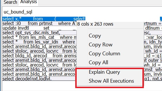
• Show all executions will show each execution.  As you can see below it provides a summary view and also the time for each execution.  It also provides contextual information about the command that executed it and also the line number in the trace file.

• Explain query will show an execution plan.  This is very useful as the explain plan is really dependent on the query with bind variables.  A common mistake is to analyze queries with bind variables replaced.  This provides a simple mechanism to get the trace

Command Analysis View

Like SQL Analysis, you can do command level analysis as well.  You can analyze the whole trace or focus on an activity.  Once you analyze you see similar output but from the point of view of MOCA commands:

You can see summary view and also similar statistics for the various commands within the analysis context.  You can for example focus in on a command that may be executed too often causing overall performance degredation.

Trace View Option

You also have the traditional option of viewing the trace file as a tree view or detailed view.  Here too we have several advantages over the competing options:

• We can look at part of huge trace

As mentioned above when we right click on an activity we can create a trace for just that portion.  That sub-trace is opened into the trace viewer:

• Ability to filter out noise

When we open a trace file, we get an option to filter out some typical parts of the trace to make it easier to view.

This will reduce the resulting view significantly as the common house keeping commands in MCS and MOCA will be ignored.  You can also put additional commands to ignore.  This also reduces the size by getting rid of some other parts of the trace.

• Tree View and Detailed View in side by side panes

Above enhancements allows us to view very large trace files in this view as well.  Then we can see the contents in two panes where right side shows it as a tree and left side as text:

• View Arguments in a tab

We can highlight a command in the tree view to see the arguments that are available to it in the Arguments tab:

• Easily see FLOW messages

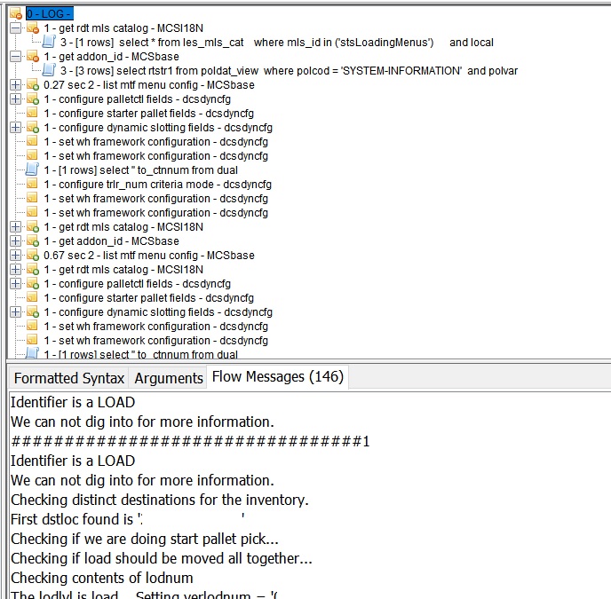
MOCA code may put explicit trace messages as FLOW type.  These provide explicit trace hints that can be valuable in making sense of a complex command.  The "Flow Messages" tab shows such messages based on the selected node of the tree:

Conclusion

RedPrairie/JDA server tracing option is very valuable and provides a tool to perform indepth analysis and troubleshooting.  Complex use cases become difficult due to the size of the trace file.  Our approach provides us a solution to focus on the problems and eliminating noise.  Our consultants are also users of our tools so this allows us to imporve these by utilizing their feedback.  If you have any questions or comments please contact us.

Is Archiving the way to deal with old data in 2018?

Overview

JDA/RedPrairie WMS requires customers to have a data archival strategy. The approach that they push and most customers end up adopting is akin to using a sledge hammer to push a nail.

The JDA approach is quite interesting and probably an appropriate mechanism if the year was 1995. Their approach is to say that the data will be archived to an identical environment from the point of view of software but that other environment will have older data.  This is a very interesting paradigm because all of the reports, queries, use cases, etc. that we may have will work in exactly the same way in the archive environment - all we have to to validate is that the data from the current system is properly moved to the archive instance.

Issues

So what is the issue with above approach?

• We are adding another environment to support.  So lets say we have 5 production environments (for sets of warehouses) - we really need 5 additional environments for archive.  Then to support testing and development we will have 10s of additional environments.  If we have some related environments like EMS, parcel, report writer, etc - those may be needed as well.
• These additional environments need to be part of the software development life cycle.  All rollouts need to go to these environments as well.
• We create "cut off" points, i.e. some queries would need to go to multiple environments.
• Some advanced use cases like "recalling" and "returns" may need overly complex solutions where we may need to query archive and online instances.
• An additional point of failure for daily maintenance.

What are my options?

So do we have any options?  First we really need to check the calendar.  What we considered as "too much data" in 1995 will be considered a "below average database size" today.  Secondly we need to understand that number of rows in a table does not cause an issues - it is the access path.  Thirdly, today's databases have advanced features like partitioning that render such complex strategies obsolete.  In this article, I will focus on solutions available in Oracle - but please note that SQLServer has similar concepts and features.

First let us firmly establish the problem we are trying to solve.  The size of the table is not a measure of performance - it is always the access path - so what we are really trying to address is data management not performance.  Another "problem" that archiving solution supposedly addresses is that queries against the archive instance will not adversely impact the online system's performance.

Data Management - Partitioning

The solution that is most promising for data management problem is to utilize advanced database feature for "partitioning" and let the data stay in the online system.  This implies that your single online instance will have all of the data all the time.  Dispatched shipments will simply be in a different partition.

Ideal partitioning solution will be to create the main partition by range (or in new versions interval partitions).  Then have a sub-partition by warehouse.  That will result in manageable data in each partition.  This partitioning strategy provides good information to the database to parallelize queries.

Data Isolation - Reporting Database

The other problem of providing an isolated environment for queries is easily addressed by utilizing the concept of stand-by database or "data guard" or "reporting databases".  Please refer to the database documentation - but what it provides is a completely isolated database instance that is "almost" up to date and can be used for reporting.  The setup is low level DBA activity and requires little application support.

But this may not be needed for majority of the scenarios.  Such a database should be made available for true research activities where we will not be using the RedPrairie/JDA client to access the tables.  All use cases where we need to access the data through application should be handled by connecting to the online instance and letting database handle the large amounts of data.

How should I partition the data?

To effectively partition we need to have a good date column on the table and for warehouse sub-partition warehouse id should be in the table.  Unfortunately some tables in JDA WMS do not have these columns so small modifications are needed to make it all come together.  

In the following section I have listed the tables and suitable partitioning keys.  Following enhancements should be done to make it all work:

1. When "shipping trailer" dispatches, update following tables with uc_trndte set to dispatch date/time.  And if table does not have a warehouse id, then we set uc_wh_id column.
• trlr
• car_move
• stop
• shipment
• shipment_line
• ord
• ord_note
• ord_line
• ord_line_note
• oub_serv_ord
• oub_serv_ord_line
• pckwrk_hdr
• pckwrk_dtl
• pckmov
• invlod
• invsub
• invdtl
• locmst
• manfst
• shp_dst_loc
• sp_hand_ref
2. When "receiving trailer" dispatches, update following tables with uc_trndte set to dispatch date/time.  And if table does not have a warehouse id, then we set uc_wh_id column.
• trlr
• rcvtrk
• rcvinv
• rcvlin
• locmst
• inb_serv_rcvinv
• inb_serv_rcvlin
3. As a general rule - use base 36 sequences

So the overall partitioning strategy will end up as follows (not including work order tables)

Table	Partition 1	Sub Partition	Online Data	Mod Needed
Transaction History Tables
dlytrn	trndte - month	wh_id - list	No separate concept
trlract	trndte - month	wh_id - list	No separate concept
ordact	trndte - month	wh_id - list	No separate concept
invact	trndte - month	wh_id - list	No separate concept
cnthst	adddte - month	wh_id - list	No separate concept
wrkhst	issdte - month	wh_id - list	No separate concept
canpck	candte - month	wh_id - list	No separate concept
pko_act	ins_dt - month	wh_id - list	No separate concept
pko_act_dtl	ins_dt - month	None	No separate concept
Workflow History Tables
cnfrm_bck_serv	moddte - month	wh_id - list	No separate concept
cnfrm_inv_serv	adddte - month	wh_id - list	No separate concept
cnfrm_noninv_serv	adddte - month	wh_id - list	No separate concept
Order Tables
trlr	uc_trndte-month	stoloc_wh_id	uc_trndte is null	#1
car_move	uc_trndte-month	wh_id	uc_trndte is null	#1
stop	uc_trndte-month	uc_wh_id	uc_trndte is null	#1
shipment	uc_trndte-month	wh_id	uc_trndte is null	#1
shipment_line	uc_trndte-month	wh_id	uc_trndte is null	#1
ord	uc_trndte-month	wh_id	uc_trndte is null	#1
ord_note	uc_trndte-month	wh_id	uc_trndte is null	#1
ord_line	uc_trndte-month	wh_id	uc_trndte is null	#1
ord_line_note	uc_trndte-month	wh_id	uc_trndte is null	#1
oub_serv_ord	uc_trndte-month	wh_id	uc_trndte is null	#1
oub_serv_ord_line	uc_trndte-month	wh_id	uc_trndte is null	#1
pckwrk_hdr	uc_trndte-month	wh_id	uc_trndte is null	#1
pckwrk_dtl	uc_trndte-month	wh_id	uc_trndte is null	#1
pckmov	uc_trndte-month	wh_id	uc_trndte is null	#1
invlod	uc_trndte-month	wh_id	uc_trndte is null	#1
invsub	uc_trndte-month	uc_wh_id	uc_trndte is null	#1
invdtl	uc_trndte-month	uc_wh_id	uc_trndte is null	#1
locmst	uc_trndte-month	uc_wh_id	uc_trndte is null	#1
manfst	uc_trndte-month	uc_wh_id	uc_trndte is null	#1
shp_dst_loc	uc_trndte-month	uc_wh_id	uc_trndte is null	#1
sp_hand_ref	uc_trndte-month	uc_wh_id	uc_trndte is null	#1
Receiving Tables
trlr	uc_trndte-month	stoloc_wh_id	uc_trndte is null	#2
rcvtrk	uc_trndte-month	wh_id	uc_trndte is null	#2
rcvinv	uc_trndte-month	wh_id	uc_trndte is null	#2
rcvlin	uc_trndte-month	stoloc_wh_id	uc_trndte is null	#2
locmst	uc_trndte-month	wh_id	uc_trndte is null	#2
inb_serv_rcvinv	uc_trndte-month	wh_id	uc_trndte is null	#2
inb_serv_rcvlin	uc_trndte-month	wh_id	uc_trndte is null	#2
Job/Task History Tables
job_definition_exec	start_dte-month
task_definition_exec	start_dte-month

Conclusion

If you have been live for some time - chances are you have experienced your share of Archiving Blues. Because of the overly complex archive solution - people often resent even going to archive instance. Volumes of priceless data in dlytrn is completely ignored and rather than valuing it we consider it a burden. Using the simple strategies described here we can enter the 21st century for our JDA WMS systems. We can consider dlytrn as a valuable data source which we choose to not purge and are not worried about it growing to 100s of millions of rows. We can utilize simple techniques like "stand-by databases" and mine through that data to see what gems may be there - or if we do not have time or budget right now at least we can leave data there rather than losing it. Also by keeping it all in one system where historical data is easily accessible we do not have to worry about untimely exceptions. If we have to print a packing slip from 5 years ago - no problem; we simply go to "Report Operations" and print it.

Integrator In-Memory Database - Makes Integration Even Easier

Overview

Recent RedPrairie Integrator versions include an embedded H2 database that opens up new possibilities for efficient and simple integration projects.  The basic components provided are:

• create internal table
• insert into internal table
• select from internal table
• This command asks for a table_name as a parameter - but we can pass a complete join clause as well.
• release internal tables

In some respects the idea is similar to caching discussed in another post - but the added functionality that helps in integration is the ability to apply complete SQL operations.

As of the writing of this blog, this functionality is less known and primarily used internally by RedPrairie integrator itself to abstract the inbound IFD as a table and for "Expression on Child Segment" IFD Field class - but it can come in handy in other cases as well.

Complex Mapping Scenario

If the inbound structure closely matches the RedPrairie concepts - then nothing special is needed - but in some cases the structures can be quite different.  In my experience the various SAP IDOCS present the data in a large number of mutually connected segments, for example:

Here the left side represents an incomplete view of a delivery in SAP.  Right hand side represents an order in WMS.  As you can see the SAP view is a lot more verbose and it needs to transform basically down to a order and order lines.

How to handle this mapping in standard integrator?

This type of mapping is not a problem for Integrator.  It has been able to handle it since the earliest versions.  Some of the tools available are;

• Ability to access any inbound IFD field as an EO Column
• Create EO segments at the same level as inbound IFD
• Using "Expression on Child Segment" concept on the final result IFD.

Some less experienced implementers end up creating intermediate tables to address this type of mapping - that is not needed.  We can map it in one shot, i.e. inbound IFD goes via EO creation to the result IFD which looks like the right hand side.

The result is that the integration works but can be a resource hog.  Basically every time an EO segment instance is created - it has to push a subset of the inbound IFD to the internal database (it used to be actual tables and now it is the embedded H2 database) and then system allows for executing SQL against it.  As described above the traditional solution would have required several EO segments parallel to the various inbound IFD segments, e.g.

Once these additional EO segments have been created - the final result IFD will use "Expression on Child Segment" to create the final fields.  Each of these IFD fields will require integrator to push the EO segment data to the internal database so that SQL can be applied.  Lets say you have 10 order line fields that have to be created in this fashion - it will require the EO data to be pushed to the internal database 10 times for the same order line.  As you can see this can quickly become a performance issue.

Internal Database to the rescue

At a very basic level - the above discussion highlights the key deficiency in integrator - that it does not allow for joining data from multiple inbound segments.  So creating the intermediate EO segments is a way to circumvent that.  Using the internal database we can overcome this and simply load the inbound IFD to internal databases.  Afterwards we can simply join the data so that the EO also matches the result IFD:

The basic difference is that we have introduced a high level segment that would load all of the relevant inbound IFDs to internal database as tables.  And at the end we would release those tables.  The retrieve method implementation of the UC_LOAD_HOST_ORD will utilize the "create internal table" and "insert into internal table" commands.  

First we need to create a component that would return a resultset for each inbound IFD segment that we are interested in. For example lets call that component "get usr sap order segments as rs". It could be implemented as:

/*
 * During integrator execution - ifd_data_ptr is on stack
 * so it does not need to parse the inbound again.  But
 * in case it is not on stack, e.g.
 * for testing then we get it via standard
 * integrator command.
 */
if ( @ifd_data_ptr#onstack )
   hide stack variable where name = 'ifd_data_seq'
else
   sl_get ifd_data_ptr 
|
{
   /*
    * If an inbound IFD is optional - we need to still
    * create an empty recordset for it
    */
    ... create empty recordsets
    |
    /*
     * Now fetch the inbound IFD Data into a
     * recorset, e.g. lets say inbound IFD
     * segment is called MYSAPHDR - we will say
     */
   {
      {
         sl_list ifd_data_fld <
         where ifd_seg_id = 'MYSAPHDR'
         >> uc_sap_mysaphdr
      }
   }
   |
   ... so on.  Get every relevant inbound IFD
   ... segment to a recordset.
   ... This step is extremely efficient as it
   ... is simply looking at parsed 
   ... view of inbound IFD from memory.  
   ... If an inbound IFD was optional, e.g.
   ... order notes - then you still need
   ... to create a valid recordset with 1 row.
}

Now we can create another command say "create usr sap order tables" as follows:

get usr sap order segments as rs
|
{
   release internal tables
   ;
   create internal table
   where table_name = 'uc_sap_mysaphdr'
   and res = @uc_sap_mysaphdr
   ;
   ... so on for all tables
}

The UC_RELEASE_HOST_ORD will simply call "release internal tables" command.

With that in place the ORDER_HDR, ORDER_DETAIL etc. will no longer utilize the generated retrieve method implementation that says "where sl_data_fk = :sl_data_pk" instead it will call a MOCA Command  that will utilize "select from internal table" to get data from multiple inbound IFD segments utilizing joins - which is extremely efficient.

This will utilize the several tables created earlier and access the data from there. It can utilize complete SQL language including group and join clauses:

{
   select from internal table
   where select_stmt =
     "select ... any columns from any table ...."
   and table_name = 
     " uc_sap_mysaphdr join .. left outer join .." 
}

Some Gatchas

• Note that the internal tables are created directly from the recordset.  If the recordset is empty, the table cannot be created as it does not have the column information.  That is why we need to have an empty table in that case.  The "sl_list ifd_data_fld" command returns ifd_data_seq and ifd_data_dtl_seq in the recordset.  So you can create the empty recordset with these values set as 0.  That way the recordset will not be empty but when you access it for the particular ifd_data_seq you will not get a row - which is what we wanted.
• If this functionality is used, then all segments below UC_LOAD_HOST_ORD must use this and not the traditional "sl_data_fk = :sl_data_pk" retrieve methods.  This is because when creating the tables we called "release internal tables" and that also killed the table that integrator had created for this SQL to work.
• Referring to first gotcha - note that in MOCA if you assign one recordset to another, it just sets the pointer and does not clone the data.  This implies that if you set multiple recordsets to the same "empty" recordset then even though you are thinking they are two different recordsets - they are really the same.  So if you move to the last row in one - you will also move to the last row in the other.  Where it would cause an issue is that when you will create the internal table from one - the next one will not work.  You will need to call ".reset" on the recordset again before using it.

Summary

The basic idea is that we should try to match event output to the RedPrairie order model via this capability.  That implies that we push the inbound data to in-memory tables once and then join them as needed to create the final set.  At a very high level the approach is similar to a two-step approach of first loading the data to temporary staging area and then logging another event from that - but this achieves that in a single step and will be more optimal - both in performance and also in management.

Right way to tackle RedPrairie/JDA Interfaces

Every WMS implementation needs to deal with interfaces.  This includes host interfaces, e.g. interfacing with SAP, Oracle, JDE, etc. and also to the automation equipment.  Many times the project plan calls for these tasks at the wrong time and that can lead to overall delays and rework.  Timing this activity correctly is critical to the overall success of the project.

Many times the customer's past experience with interfacing influences their decision to start interface discussion prematurely - but such proactive approach is not helpful.  So one thing we need to establish upfront is that RedPrairie/JDA will be able to handle any type of interface requirement.  If you can send it RP can process it! So do not lose your sleep over it.

Abstraction is the key

We need to understand that the actual project is WMS implementation and not the interfaces.  Interfaces need to be understood abstractly as just another mechanism to provide data.  Nothing more and nothing less.  So once it is established that RP can do any type of interface work then we need to focus on WMS solution summary and not interfaces.  

Proper place for Interfaces in the Project Plan

At a very high level, the project plan should be as follows:

1. Key customer resources get trained on the solution set.
2. Software is installed in development environment
3. A Proof of Concept exercise is done with standard solution
1. This highlights the interfaces
4. A solution summary is developed
1. Interfaces are called out here
5. Interface Discussion

A completely wrong approach will put the interface discussion ahead in the plan.  I have seen instances where the interface discussion is done even before the software is installed.  Such meetings are not very productive because the customer's resources do not understand RP and the implementer does not understand customer requirements - so as a result a sub-par interface diagram is created.

Host Interface Matrix

Host interfaces are simply a mechanism to provide data to RedPrairie.  It is not different from manual data entry from that aspect.  Solution summary should be firmly established before this discussion starts.  One way to approach this is that the customer could simply take screenshots from RedPrairie client and highlight the data that they expect to come from a host system - that will be easier than going through spreadsheets with cryptic column names.  Any RP implementer should be able to take such a document and convert that to an actual interface.

Similarly for data going to host, the customer SME (Subject Matter Expert) can highlight the data that they would expect to populate the host system.

MHE Interfaces

MHE (Material Handling Equipment) interfaces are no exception.  The full solution summary should first describe the use cases in terms of RF flows.  This should be done even if majority of the picking is done by MHE.  This provides a baseline for testing.  Once this is done, MHE use cases should be defined and an equivalence diagram should be created.   This diagram will describe how MHE picking, for example, is equivalent to RF picking.  A diagram like this will form the basis for MHE interface discussions.  This will also help during development and unit testing phases.

MHE Emulator

Ability to emulate MHE messages is key to a successful implementation.  Unfortunately many MHE systems do not provide such capability.  This becomes a challenge if MHE system communicates over sockets.  A simple emulator can be created by RedPrairie integrator where you can create a system that represents the host system and listens for messages.  You can verify MHE protocol in this way.  You can use similar techniques to send completion messages back to WMS. 

When sending data to MHE, typical triggering point is the pick release process.  pckwrk table(s) should form the basis for data that is sent to MHE for picking.  Custom columns can be added here to incorporate any unique concepts but this should generally be the starting point.

The transactions back from MHE will typically call a flavor of "move inventory".  If we have an equivalence of these use cases to RF screens then this can be a relatively simple exercise.

Another approach may be to have a folder with raw messages and create a simple groovy command that sends data from this folder to the WMS.  You can also use "telnet" to send data.

Interesting WMS Concepts for MHE

RedPrairie WMS provides several concepts that can form the basis for providing data to MHE at proper level.  Often I have seen that new concepts are introduced in this regard which adds needless complexity and testing headaches:

• Idea of picking cartonization
• Idea of lists that can group cartonized cartons
• Non cartonized picking directly to a tote
• Pick Release process and associated standard triggering points like "register picks released"
• Replenishment Configuration concepts

For most picking systems, e.g. Pick To Light, the MHE system will have a location table with similar locations as RedPrairie.  Inventory levels in RedPrairie will be assumed to be accurate as well.  In such systems orders are allocated within RedPrairie and at pick release time we send data to the MHE system.  RedPrairie concepts are a "shoe in".  By the time pick release is done - we know exactly which carton needs inventory from which MHE locations so appropriate messages can be constructed.

When MHE system completes a pick - some systems will tell exactly what was picked while some will simply say "this tote is picked".  In either case - processing of such a message should simply call "move inventory".  Sometimes implementer would make this interface needlessly complicated by a false assumption that "move inventory will be too expensive".  This unproven and untested notion will then translate to new concepts and make the whole implementation overly complicated.  It is always best to not over-engineer this step and simply pick the inventory in RedPrairie when it is picked in MHE.

MHE system from this point on may have multiple stops, e.g. audit station, weight station, etc.  Such locations may be handled as simple P&D locations or hops.  In either case - if MHE system can send a message in these cases - that message should translate into a "move inventory" call.  Refer to this article if you have a use case where certain percentage of totes need to be audited.

Every implementation may be slightly different but always have following goals:

• Do not invent new concepts
• Always equate to corresponding RF use cases

Summary

Interfacing capabilities are a strong suit for RedPrairie/JDA WMS systems.  Do not let some bad past experiences influence the project plan too much.  Considering interfaces as just another type of data entry method simplifies the project a great deal.  Based on the type of implementation - you may need significant hours, but those should not translate to significant complexity.  Proper abstraction that preserves the core RedPrairie concepts will go a long way.

Caching Data Using MOCA

Overview

We often need to cache some data during any implementation.  If you are creating a C component, that may take form of a "static" variable.  You could sometimes use "session variables" - if intended scope is a transaction.  You could also employ "Environment Variables". 

RedPrairie software itself utilizes caching in several algorithms.  Most of the implementations use C static variables.  This path is fine but requires a lot of housekeeping code and also prone to bugs - especially memory leaks.

As of 2011, MOCA has introduced external caching.  One such caching provider that MOCA supports is "infinispan".

Possibilities

This opens up some very interesting possibilities.  In this blog, I will describe a solution that we incorporate in almost all of our implementations, i.e. we cache results of an arbitrary MOCA command such that if the same command is called again - it simply returns data from the cache.  The solution is quite simple - thanks to the wonderful concepts implemented in MOCA.

MOCA Command "execute ossi moca and cache"

Whenever we need to call a command whose result can be cached, we execute it via this interface.  It is similar to the "execute server command" MOCA command - but the difference is that the results can be cached and if called again, it will return data from the cache.

It has following input parameters:

Argument	Description	Comments
uc_moca_cmd	This is the exact command that needs to be executed	Similar to what you will pass to execute server command
uc_inline	Should the command have access to stack variables?	Similar to "inline" parameter of execute server command
uc_cache_key	The results of the execution will be saved in cache with this key	This will include some key data for the execution so that it can be looked up again. You could default it to MOCA command itself but that will not work very well for inline contexts. Most of the time you can come up with primary key of this cache node. For example policy table primary key or area key etc.
uc_cache_grp	The cache can be made up of several groups	For example policy caches can be placed in one group, areas in another

While such caching is often very useful in production environments - it can be a pain in development environment where we are frequently changing the data that is cached.  That is why it is a good idea to support an environment variable to disable caching.  When the caching is disabled - this behaves exactly like "execute server command".  A sample implementation may be as follows:

publish data
where uc_inhibit_ossi_cache = @@UC_INHIBIT_OSSI_CACHE
|
if ( @uc_inhibit_ossi_cache = '1' )
   execute server command
   where cmd = @uc_moca_cmd
   and inline = @uc_inline
else
   execute ossi moca and cache core

MOCA Command "execute ossi moca and cache core"

This is the main command that utilizes the caching functionality in MOCA.  It works off the same input as the above command.  It first looks up the the cache for the passed in key.  If found it returns the complete result set from the cache.  If not found - it will execute the command, put the result set in cache and then return the data.  A sample implementation may be as follows:

publish data
where uc_my_infispan_cache = nvl(@uc_cache_grp, 'OSSI__MISC' )
and   uc_my_inline = string ( nvl(@uc_inline,0) )
|
{
   [[
   import com.redprairie.moca.cache.*;
   import com.redprairie.moca.cache.infinispan.*;
   //

   // This creates the cache.  Each cache group becomes a different cache.

   //
   MocaCache cache = CacheManager.getCache(uc_my_infispan_cache, 

                        new InfinispanCacheProvider(), null, null); 
   //
   // First get the cache_key from the cache.  We always put the full resultset in cache

   // so the get is expected to return that.
   //
   my_rs = cache.get ( uc_cache_key );

   //

   // If we do not find resultset in cache - then we execute the command (inline or not)

   // after executing, we put the whole result set in cache

   //
   if ( my_rs == null )
   {
      if ( uc_my_inline == "1" )
         my_rs = moca.executeInline ( uc_moca_cmd )
      else
         my_rs = moca.executeCommand ( uc_moca_cmd )
      //
      cache.put ( uc_cache_key, my_rs );
   }

   //

   // If we found in cache or executed - by this time we have the resultset

   //
   [ret:my_rs]
   ]]
   |

   //

   // we publish the resultset
   publish data combination
   where res = @ret
}

Use Cases

This comes in quite handy.  For example in complex integration projects we often have lookup tables - this improves the performance significantly in that case.  Similarly data in policies, area, storage polices, pick policies, etc. is quite static and can take advantage of this capability.  

In addition to this, this method makes the concept quite abstract and requires minimum housekeeping.  All we need to do is construct the command and execute it.  MOCA allows the whole recordset to be cached so we can thus cache complex information.

Additional Documentation

For additional features and detailed documentation, refer to "MOCA Developer Guide" chapter on "Caching"

Myth Buster - Number of rows in a table is not the issue

Overview

I have heard this myth so many times that we have issues "because we have too many rows in table x" - or in response to a support request we are told "this is because your purges are not set up properly" or over engineered solutions are created because "pckwrk has too many rows".

Note that number of rows in a table is never the issue for performance - it is the access path to the data.  Furthermore in a system like RedPrairie WMS (an On Line Transaction Processing System) - most of the data is coming from the database cache so it is absolutely not an issue!  This also goes into a tangent that on Oracle do not spend so much time in distributing your tablespaces to different disks - this is not 1995!

Current version of this article relies on data from an Oracle database but for this discussion, same concepts apply to SQLServer.

What is a table?

A table, from the point of view of the database, is not a monolith where you read it from top to bottom to see where your data is.  It is made of segments that are made of blocks.  You simply need to get to the right segment and block to read your data.  You get there through the use of data dictionary and indexes.

So from the point of view of the overall access path, if you divide your 10 million row table into 10 tables and you look at some "index" to see which table you should go to and then go to that table - your overall solution will be no better than going at the 10 million row table itself.

Data partitioning for extremely large tables is very useful and I am not disputing that.  There are other reasons to split the data - not performance in an OLTP system.  

Index Depth is the key

Oracle uses a variant of a B-Tree index.  The key concept here is the "height" of the index.  Height represents how many reads are needed in order to get at the desired data block.  Even if you have 10 million rows in a table, your height should be <= 3.  That is pretty good and should not cause any performance issues.  While we are at it - lets bust another myth - it is not necessary to rebuild the indexes due to performance issues.  This is because the B-Tree is balanced as the data is inserted - It is not 1985!  Every time you rebuild an index for gaining performance an engineer at Oracle/Microsoft gets heart burn.

To see the index height, analyze the index in oracle and then see the BLEVEL column in "ind" view.  Actual height is that number plus 1.  You will rarely see this value > 2.

Putting the concept to test

Following tests are on a development machine that has not been tuned for production use.  I am comparing the performance to access a table by PK between two tables that have very different sizes.

• dlytrn has 17,471 rows.  The BLEVEL is 1 for the primary key.
• usr_large_dlytrn has has 626,542 rows. The BLEVEL is 2 for the primary key.

Access Times for dlytrn (same PK accessed multiple times)

1. 1,000 - 2.4s
2. 10,000 - 14.29s
3. 100,000 - 127.88 s

Access Times for usr_large_dlytrn (same PK accessed multiple times)

1. 1,000 - 1.69s
2. 10,000 - 9.92s
3. 100,000 - 104.54 s

So in this test the larger table gave better performance - but that is not important.  It may have given better performance because of other reasons.  The key message is that number of rows in the table itself had no effect - especially in an OLTP system where our queries typically return a very small percentage of the rows in a table and that access is through indexes and cache.

But I swear - when we had performance issues last year and we deleted data from pckwrk - things improved!

I believe you - but unfortunately when someone faces acute performance issues, we often forget about basic troubleshooting strategies and start "trying out options" - sometimes expensive options without any basis for supporting them.  For example people would right away suggest "rebuild indexes" and "purge" without any evidence to support their decisions.  And when such actions are taken we often do not capture the results objectively.  For instance if we rebuild, we should see if IND view on oracle shows any improvement.

When you purged data in pckwrk, most likely the access path to pckwrk changed and that is what improved your performance - not the number of rows.  So in that case we should have identified the problem query and analyzed its query plan.  If we analyzed the same query after purging the data we would have noticed a different plan.  Had we used the improved plan on the larger table - we would have seen the same improvement.

Right Indexes vs More Indexes

In many cases dropping some indexes can improve performance as well.  We have several indexes delivered by standard product that simply do not make any sense.  On top of that several projects end up creating many more indexes without analyzing the need - and those indexes are often the culprit when we are seeing the performance issues.  For example if you add an index on wh_id column in pckwrk by itself - that will hurt performance.  We should add indexes only when they are selective enough to give less than 10% of the rows.

Bind Variables

MOCA "auto binds" the SQL statements, i.e. if you ran a query [select * from pckwrk where pcksts = 'P'], MOCA will run it as [select * from pckwrk where pcksts = :1].  So whereas with [P] Oracle had enough information to understand that an index on pcksts is good when Oracle does not know the value (as in running with :1) then Oracle may decide that 99% of rows in pckwrk have same pcksts - so maybe it is not a good idea to use pcksts index.  These are the types of situations where deleting rows from pckwrk may help because pcksts then becomes more selective - but as pckwrk will grow again the same issue will re-appear.  As of 2011, MOCA provides a "#nobind" hint.  If that were used for the query then Oracle will run it without bind variables and make the correct decision.

Adding more columns to an index

This is a less known strategy and often has extremely good results.  As tables grow organically, even for a selective index - database needs to access several rows in the base table in order to get additional information.  For example lets say we got 100 locations and we join to inventory tables and the query may need invlod.loducc.  In order to get that one column, database will need to access the invlod table in addition to the index on invlod.  The resulting overhead may be very low but often such queries are running 100s of times within a transaction so that number can add up.  An explain plan would have looked good but would include "TABLE ACCESS BY ROWID FOR INVLOD".  That can be an issue.  If you modified the index definition to include the columns that your query needed, then accessing index will be enough and the improvement will be quite significant.

Joining with views in general and poldat_view in particular

As indicated in Top 10 mistakes, policies are often over-used and we end up with unbalanced data distribution.  So even for a given polcod, polvar, polval - we may not gain good selectivity.  That coupled with the complexity of the poldat_view where it is trying to add rows for each wh is often a major problem.

If you are about to put a join to "poldat_view" in your query - stop, take a glass of water and try to think of some alternate strategies.  Even though joining is always faster than using "|" and do multiple queries, if poldat_view is involved - it may be better to not use join and go for "|" and a second query to get data from poldat_view.  Another option may be to read the poldat_view first into a recordset and then access that within the loop of your query.

If you must use poldat_view, then see if using base poldat is an option.  For example if your data is always expected to be warehouse specific, then you could use poldat.wh_id_tmpl of the actual warehouse.  

Any time you use views in the query - and especially poldat_view - always explain and also see if the database could run it incorrectly under certain scenarios.  I generally favor not joining to the view, especially poldat_view, and use one of the other strategies.

Changing Query Plans

Often when our symptom is "Performance was fine yesterday" - the issue is that some change in data distribution caused the database to start using a different plan.  In such situations, it helps to see the problem query and see its plans historically.  Then we should pin the plan that was running well.

Conclusion

Purging data is not a bad idea and we should have an appropriate purge and archive strategy but that falls in the domain of "data management" not "performance management".  Number of rows in a table is not a measure of performance.  When faced with performance issues, it is important to understand why we are facing the problem and then take corrective action.  Every corrective action should then be scrutinized to see if it really helped or had no effect.  An incorrect assumption can become a problem over time because then when we try to do things right - there is resistance that suggests that all of these changes were made to improve performance.  So key message is:

• Just number of rows in table is not a measure of performance
• Do not create complex solutions where you try to "not use pckwrk because it has so many rows".
• Do not worry that prtmst has 1M rows.
• Rebuilding indexes will rarely - if ever - help performance
• For RedPrairie WMS, data is accessed mostly by indexes and cache, so do not over engineer data distribution strategy where you try to put tables on different physical disks.  You have bought that expensive disk array - let it do its job!
• When faced with performance issues, always look at the query plan (and with bind variables).  See older plans and see if execution plan changed.
• Remove unnecessary indexes.
• Employ change management regime to control the changes done due to performance issues.  Capture the improvements objectively.

RedPrairie Implementation of Sampling in Workflows

Sometimes you come across an algorithm that is so elegant yet simple that you have to appreciate it.  It is a common requirement to apply some operation to a percentage of tasks for audit reasons.  For example you may want to divert 10% of the picked cartons to a special lane for audit.  Similarly you may want to apply some workflows to a certain percentage of items only.

When I considered the problem, I concluded that I would have to somehow mark the task, e.g. pckwrk, to indicate which cartons need to be audited.  RedPrairie has the concept of Workflow Rates:

Looking at this setup I was intrigued because the setup was independent of any workflow and was talking about probability.  Going deeper into the implementation, I was amazed at the elegance and simplicity of their implementation - rather than marking every nth row and deal with the associated complexities - simply roll a dice - if it says "1" - apply workflow - Genius!

Consider that if we have a work-station next to a conveyor where picked cartons are traveling and it is the job of the user to audit 50% of the cartons that pass next to him.  He could try to pick every other carton or he could simply flip a coin when he sees a carton - heads audit it, tails let it go.  Law of Large Numbers guarantees that  our results will approach the desired rate.

How do we toss a coin in software?  Generate random numbers.  For the random numbers generated by software  each number in a given random sequence had an equal chance of occurring, and that various other patterns in the data should be also distributed equiprobably.  So all we have to do is generate a number and check against defined probability to see if we should perform the operation.

To see it working - the command responsible for doing this is "get probability calculation".  You should pass in prob_qty and max_prob_qty.  For example for 10% probability you should pass in 10 and 100 respectively.

To test it, you can run it for large numbers and see the results.  So lets run it for 10, 100, 1000,and 10000 iterations and see how many workflows we will do.  Results were - as expected:

When you run the test, the exact counts will be different but they will approach the desired 10% result.  Simplicity of this solution is truly elegant.  The result should be acceptable for anyone.

For reference, the code to generate the above table is:

do loop where iterations = 4
|
{
   sl_power
   where num = 10
   and power = @i+1
   |
   publish data
   where max_iterations = @o_value
   |
   {
      do loop where iterations = @max_iterations
      |
      {
         get probability calculation result
         where prob_qty = 10
         and max_prob_qty = 100
         and invtid_num = 1
         |
         if ( @result = 1 )
            filter data where moca_filter_level = '1'   
      }
   } 
   >> res
   |
   publish data 
   where max_iterations = @max_iterations
   and cnt_work_done = rowcount(@res)
}

Dealing with very large trace files

Overview

In RedPrairie, we often have to analyze trace files.  The trace files are generally very helpful because nothing is missed when you trace everything - but that also implies that nothing is skipped.  This means that it is not a surprise to get a trace file that has several million lines.
Most new MOCA Clients have nice trace viewers but they all have a problem with extremely large trace files.  Also the analysis is quite difficult.

Solution.

One solution is to load the trace to the database.  With a proper schema that represents the trace the analysis can become manageable.  Following tables represent a possible schema:

usr_temp_cmd_trace_analysis

Column	Specification	Comments	Example
uc_trace_file	String(500)	Name of the trace file	/blah/trace.log
uc_cmd	String(4000)	Command Name	USRint/list order lines available for wave planning
uc_lvl	String(100)	Command Stack Level in trace	1
uc_start_ts	String(100)	Start time stamp from trace	17:15:32,571
uc_end_ts	String(100)	End time stamp from trace	17:15:34,059
uc_elapsed_ms	Float	Elapsed time of this command execution	1488
uc_start_line_num	Float	Starting Line Number in trace file	202
uc_end_line_num	Float	Ending Line Number in trace file	121208
uc_args	String(4000)	Pipe separated List of arguments and values	|wh_id=xyz(STRING)

usr_temp_sql_trace_analysis

Column	Specification	Comments	Example
uc_trace_file	String(400)	Name of trace file	/blah/trace.log
uc_bound_sql	String(4000)	SQL Statement with bind variables	select super_usr_flg from les_usr_ath where usr_id = :var0
uc_unbound_sql	String(4000)	SQL Statement with bind variables replaced with values	select super_usr_flg from les_usr_ath where usr_id = 'XXX'
uc_rows_returned	String(100)	# rows returned	1
uc_elapsed	String(100)	Elapsed Time in seconds	0.002135123
uc_line_num	Float	Line Number in trace file	377
uc_cmd	String(4000)	Command that called this SQL	MCSbase/list users
uc_lvl	String(100)	Command Stack Level In Trace	10
uc_cmd_start_line_num	Float	Starting Line number of this trace file	352

Loading the trace to these tables

Simple MOCA command can be developed to read the trace file and load these tables.  The latest version of Oracular MOCA Client will include this functionality as well.  Since the trace files can be very large, you should use groovy to read the file - as opposed to using "read file".  Additionally you should commit the data as it is being loaded into these tables.

Typical Analysis

Once data is loaded into these tables analyzing huge trace files becomes quite manageable, for example:

• Using usr_temp_cmd_trace_analysis, you can pin point which execution of a command took the longest, i.e. highest value of uc_elapsed_ms.
• usr_temp_sql_trace_analysis.uc_bound_sql has bind variables so it can help in analyzing SQL statements that are executed very frequently.  You can group by this column and sum uc_elapsed and take count(*).  This way it becomes easy to find SQLs that are executed very often.
• usr_temp_sql_trace_analysis.uc_bound_sql can be explained to see how the statement will be executed by the database.
• By comparing the total time in usr_temp_sql_trace_analysis and usr_temp_cmd_trace_analysis, we can find out if the performance issue may be external to the database.  For example if usr_temp_cmd_trace_analysis shows 2 minutes but the total time in usr_temp_sql_trace_analysis  is 1 minute, we know that 50% of the overhead is outside the database.
• If we see that a command is executed very frequently, according to usr_temp_cmd_trace_analysis, some caching techniques may be employed or the commands may be disabled.

We will add some of these features to future versions of Oracular MOCA client.

Conclusion

RedPrairie trace files can quickly reach millions of lines.  For example tracing of wave planning, pick release, allocation, etc. can often create huge trace files.  Analyzing these via typical tools can be very challenging.  By loading the data into a database table, we can pin point the problems very easily.  The script to load the trace into the database can be quite efficient.  I have loaded a 7 million line trace file in around 30 minutes into these two tables.  Once the data is loaded we can easily find the problem areas.

Dealing with characterset issues

Overview

Recently I was involved in a project where we had to call a web service (XML post over http).  The data in RedPrairie database was in UTF8.  The special characters in this case were Turkish characters.  In this post I will document the various issues we faced and how I addressed them.

Understanding the environment

When dealing with international charactersets, I have seen that most often the parties involved do not completely understand what they are talking about and that can often hinder progress.  Following are some simple scripts to get some basic data:

• What is the database characterset?
On Oracle execute:

[SELECT * FROM nls_database_parameters where parameter = 'NLS_CHARACTERSET']

Typically you will see something like AL32UTF8 implying UTF. Refer to oracle documentation for other charactersets.
• How is it translated within RedPrairie technologist stack?
When the string is read into a Java String, you can ignore what Java stores it internally as. You are basically trusting Java that it knows what the string really is. If the string goes from Java to C, C will see it as a UTF8 byte sequence.
• How does the other system want it?
For this project, the other system did not understand what characterset they expect. Something like this can become quite frustrating but in situations like this you may have to simply try the various encodings.

Solution Overview

Our scenario was as follows:

1. The data is fetched
2. An XML message is created from the data
3. The XML is posted to the other sever.
4. The other system responds.

When data is fetched and converted to XML, at that time I created a file using "write output file".  "write output file" is a C component and that showed the byte sequences as UTF-8.  When that data was posted to the URL, the other side was unable to parse it.  Even though network trace showed the correct byte sequences.  You can also use groovy to write files but in that case you should declare what characterset you want the file to be in.

The other system indicated that their native characterset was ISO-8859-9 so I tried converting the XML message to ISO-8859-9 before sending.

After that is resolved, we still need to understand what characterset their response comes in as.

So the code to write out to the URL and convert the characterset will be:

/* Note the iso-8859-9 here */
publish data
where uc_rp2outside_charset = "iso-8859-9"
|
publish data
where url = 'http://whatever.com'
and body = 'xml string that has international characters.  Dont care 

about characterset here because trusting Java to represent correctly'
and uc_content_type = "text/xml;charset=" || @uc_rp2outside_charset
|
[[
URL my_url = new URL(url);
HttpURLConnection conn = (HttpURLConnection) my_url.openConnection();
conn.setRequestMethod("POST");
conn.setRequestProperty("Content-Type", uc_content_type );
//
DataOutputStream wr = new DataOutputStream(conn.getOutputStream());
// This is where we are declaring that our writer should be writing in 

// a speciic characterset
PrintWriter out = new PrintWriter ( new OutputStreamWriter ( wr, 

                                    uc_rp2outside_charset ) );
//
// This println will convert body from internal java representation 

// to the target characterset
out.println(body);
out.close();

]]

The response from the webservice will be in a specific characterset as well and we need to interpret it as such.  In this situation, after some analysis I determined that the response from the webservice was sending the data in UTF-8.

publish data
where uc_outside2rp_charset = "utf-8"
|
[[
... code to write on the url ...
DataInputStream ir = new DataInputStream ( conn.getInputStream() );

//

// This declares that the response stream from the request will

// send UTF-8.  This causes the "ret" to properly convert from

// utf-8

//
BufferedReader in_reader = new BufferedReader( new InputStreamReader( ir, 

                               uc_outside2rp_charset ) );
//
while ((inputLine = in_reader.readLine()) != null)
{
   ret.append ( inputLine );
}


]]

Conclusion

Dealing with characterset issues often becomes a challenge because most people do not fully understand the details and underlying concepts.  In such situations you may have to try some approaches, for example:

• Understand that whenever you write out or read from a connection, data may need to be converted to a different characterset.  By having some policy or environment variables, you can easily try different conversions.
• Have the ability to create files with the request and response.  
• Look at the generated files in hex editor to see what bytes are being sent and received.
• A network level trace can help as well to ensure that what is on the wire is proper character sequence.
• Many technologies show "?" to represent characters that they do not understand; for example Oracle will show "?" and so would some java technologies.  MOCA trace will also show "?" - that can throw you off because the other side may be seeing "?" and so does MOCA trace on your side - but the raw data was correct from your side.  So having a raw file helps.  When creating such raw files same concepts apply, i.e. you will have to declare what characteset the file is in.
• I have seen that ISO-xxxx-y charactersets are used more often that UTF especially on windows based systems, so if other side is not making sense, try out the appropriate ISO characterset.

Customizing RedPrairie RF Forms (Java Based)

Customizing RedPrairie RF Forms

Java Based MTF Forms

Overview

As of version 2009, RedPrairie uses Java to provide RF forms.  The underlying engine is called "MTF" (Mobile Terminal Framework).  These applications are VT based applications that may be accessed via telnet or ssh protocols.

Deployment Architecture

1. A MOCA task exists for each vendor and warehouse combination.  The task listens on a specific port and for a specific protocol (i.e. telnet or ssh).  One task serves a single vendor (e.g. LXE, Intermac, or Default) and a specific warehouse
2. The task also points to a MOCA connection URL.
3. Clients connect to the specific task using ssh or telnet protocol
4. If the vendor setup is defined correctly, the form will go directly to the login prompt and device identifier (devcod) will be determined based on RF Vendor setup.  If not defined (e.g. DEFAULT vendor), then system will prompt for a device.  This device is determined based on setup in "RF Terminal Maintenance"

Software Layout

"MTF" is a separate software component similar to MOCA, MCS, SAL, DCS, etc. and exists at the same directory level.  This component is the underlying engine that runs MTF.

The actual forms are provided by the component that uses it, which by default is "DCS" and when we have some customized forms then also "LES".

Within each component that uses MTF, the objects exist in mtfclient/ sub-folder.  The whole solution is compiled using "ant" which works off a file called "build.xml" in $LESDIR.

Within LES folder, the customized objects will exist in "mtfclient\src\java\com\redprairie\les" sub-folder and in that folder you can have one or two sub-folders that represents the customized objects:

• formlogic 
• mtfutil

formlogic folder has the forms and mtfutil is needed for common classes. 

RF Form Invocation Mechanism

When MTF calls a form, it uses the "createFormLogic" method, e.g:

As you can see we are calling it by a name and not invoking the java class directly.  This setup is in rf_frm_mst table:

The custom entries have cust_lvl of 10 and the frm_cls points to the actual class path.  You can see how this mechanism allows for overriding standard forms as well:

Creating a new RF Form

So creating a new RF form is quite straight forward, given that you know the underlying mechanism for creating the required java objects.  You will put the new form in the formlogic folder and compile the code.  You will put that in the desired menu and give the permissions to the appropriate roles.  When MTF needs to invoke the form, it will use the rf_frm_mst data to find the highest customization level and instantiate that class.

Overriding Standard Forms

This is the main reason for this blog.  I have seen far too many cases where the override is done by straight copy/paste of standard code and then modifying a few lines of code for the enhancement.  Anyone who understands basic OOP principles will get a heart burn by reading this but unfortunately far too much code exists like that.  Just look in your installation in this folder and see code like "PickupA.java", "DepositA.java", etc. and if that code is based on straight copy/paste of standard code - you are a victim of this practice.  This basically implies that in case of a version upgrade, java is not going to help - you will have to retrofit these forms and somehow obtain the new source code.

Overriding Standard Forms - The Right Way

There is no advantage of using Java in MTF if the language is not utilized fully.  Sure, java syntax is more mature than old RF forms but if you see the code there is really one to one correspondence - actually RedPrairie provides a converter that can take the old "rdt" files and convert them to "java" files.

The advantage is only if "java" is utilized fully.  As always, the RedPrairie architecture is not at fault.  Just like MOCA, MTF framework supports the "right way".

Lets say all you want to do is that when "DepositA" is invoked, it should do something different in "formEntry" than what it does right now.  You can see what it does right now by looking at MTF and MOCA traces.

So the right approach will be to do just that and nothing more:

• Create your class as an extension of the base form

• Then override the method that you did not like

Here "formEntry" and "formExit" represent overridden methods that can have any code that you want.

• And then add an entry to "rf_frm_mst" to call "UsrDepostA" when DEPOSIT_A is called.

Overriding Methods In CWmdMtfUtil

This class is provided by DCS component and it contains several utility methods that are called by various forms.  For example when directed work form is invoked, it calls "getWork" method from this class.  

This class does not have a simple mechanism like forms, i.e. there is no table where we can put our class path so that RedPrairie invokes that instead of this class so this is a bit tricky!

When a form needs to call a method from this, it will have code like:

So what we want to do is put our extended class in this session map.  If we can do that, the concepts described above would work.  So our approach will be:

• Extend the CWMDMtfUtil class

• Then override what you did not like

• And then find a suitable point where we can replace the session map with our object.  A reasonable location may be the undirected menu.  Undirected menu will be overridden using technique described above.

And thats it - now when we go to the undirected menu, after displaying it, it will replace this session variable and from that point on our override method will be invoked.

Conclusion

Cut/paste approach is often employed when modifying the Redprairie code.  This problem exists at all levels - for example the "libsrc\varint" folder sometimes contains large C files with names like "trnAlloc.c" - that is a huge concern because that is core of RedPrairie and if that is customized say good bye to easy upgrades. 

Same issue manifests at RDT level and GUI level.  Even though RedPrairie architecture is almost perfect to support extensions, implementations are often sub-par.  Customers should closely watch what objects are part of the rollouts they receive and if standard objects are being modified a red flag should be raised right there.

We have been able to successfully implement complicated enhancements without touching the underlying standard code.  There could be situations where the only solution is to modify the base code.  In those situations it is better for the customer to give up on the enhancement or come up with some compromise where the base code does not need to be touched.