Huge Trace Files - Not a problem!

Overview

JDA/RedPrarie has a very useful feature that allows for detailed tracing of a server component.  It provides information about every single server component, parameter, and also all SQLs that are executed.  But that also ends up being an issue as the traces would often reach several gigabytes.  Analyzing them becomes a problem.

Our Solution

Oracular (http://www.oracular.com) has created a client software that allows for executing MOCA commands.  It can be downloaded from http://autoupdate.oracular.com/mocaclient/ .  We have incorporated an advanced Trace Viewer into this application that allows for analyzing such trace files.  The concepts are based on some of the concepts described in my earlier blog.

Database Trace Option

When you have our MOCA Client, you can access the "MOCA Log" pulldown menu:

As described in the earlier blog post, we will be pushing the trace to a set of tables in the database.  So in the screen you can press the button to create the tables on the instance.  This needs to be done only once.

Now you can choose the trace file you want to load from the instance by pressing the insert button.  There is no upper limit on the size of trace file.  You will be able to process several Gigabyte trace file and the client will give you progress update.  Once the trace file has been parsed the parsed view is stored in a set of database tables so re-analyzing it does not require re-parsing.

The parser views the trace file as having three high level perspectives:

1. Activity.  This is from the point of view of a client that accessed a service provided by MOCA
2. Commands.  These are the various MOCA commands
3. SQLs.  These are the SQL statements that are executed

Activity View

As you select a trace file from the top grid, the various Activities will be displayed in the order of execution along with the time spent on each:

You may sort the grid as you see fit.  Each row here implies an interaction from the client (e.g. RF or GUI user) with the MOCA server.  Being able to view this is a huge benefit when trying to make sense of huge trace files as our interesting area may be one of several activities.  As you can notice that the client makes several calls to the MOCA server for house-keeping activities which create a lot of noise to filter through.  You can right click on any row here and export just that part of the trace file:

The exported trace file can be processed in any way you like, i.e. in a trace viewer of your choice.

Here you have two tabs "SQL" or "Commands" to do further analysis:

You can choose a tab and then press "Analysis" button.

SQL Analysis View

You can perform the analysis of the whole trace file or of a certain activity.  You decide that based on the filter section:

This shows a grid that has all SQLs within the context.  The SQLs here are the ones with bind variables.  This implies that we group like SQL statements.  This is extremely helpful when we are looking at a trace from the point of view of performance tuning:

You can sort the data as you see fit.  For example while looking for performance imporvements, sorting by tot_elapsed can be quite helpful.  There is also a summary section to separate the tracing overhead from the execution overhead.  The above example highlights that there is a single SQL statement that took 8 seconds.  But also that the seond one is executed very frequently and even though each execution was sub-second (0 ms to 101 ms) adding them together comes to 1.5 seconds which can be significant when looking at a transaction like inventory movement.

You can right click on any row here to see further options:

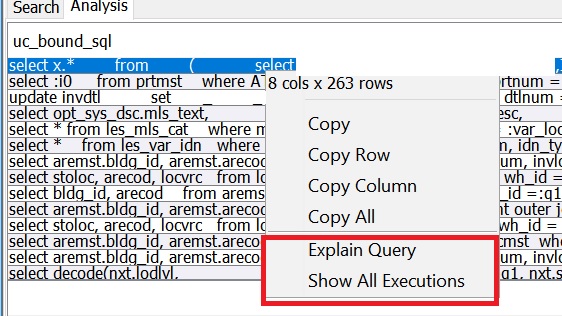
• Show all executions will show each execution.  As you can see below it provides a summary view and also the time for each execution.  It also provides contextual information about the command that executed it and also the line number in the trace file.

• Explain query will show an execution plan.  This is very useful as the explain plan is really dependent on the query with bind variables.  A common mistake is to analyze queries with bind variables replaced.  This provides a simple mechanism to get the trace

Command Analysis View

Like SQL Analysis, you can do command level analysis as well.  You can analyze the whole trace or focus on an activity.  Once you analyze you see similar output but from the point of view of MOCA commands:

You can see summary view and also similar statistics for the various commands within the analysis context.  You can for example focus in on a command that may be executed too often causing overall performance degredation.

Trace View Option

You also have the traditional option of viewing the trace file as a tree view or detailed view.  Here too we have several advantages over the competing options:

• We can look at part of huge trace

As mentioned above when we right click on an activity we can create a trace for just that portion.  That sub-trace is opened into the trace viewer:

• Ability to filter out noise

When we open a trace file, we get an option to filter out some typical parts of the trace to make it easier to view.

This will reduce the resulting view significantly as the common house keeping commands in MCS and MOCA will be ignored.  You can also put additional commands to ignore.  This also reduces the size by getting rid of some other parts of the trace.

• Tree View and Detailed View in side by side panes

Above enhancements allows us to view very large trace files in this view as well.  Then we can see the contents in two panes where right side shows it as a tree and left side as text:

• View Arguments in a tab

We can highlight a command in the tree view to see the arguments that are available to it in the Arguments tab:

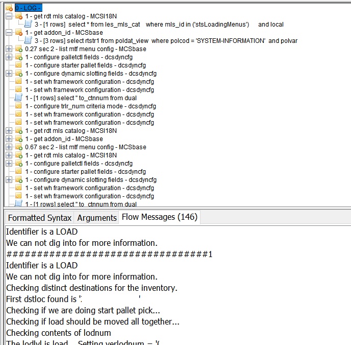
• Easily see FLOW messages

MOCA code may put explicit trace messages as FLOW type.  These provide explicit trace hints that can be valuable in making sense of a complex command.  The "Flow Messages" tab shows such messages based on the selected node of the tree:

Conclusion

RedPrairie/JDA server tracing option is very valuable and provides a tool to perform indepth analysis and troubleshooting.  Complex use cases become difficult due to the size of the trace file.  Our approach provides us a solution to focus on the problems and eliminating noise.  Our consultants are also users of our tools so this allows us to imporve these by utilizing their feedback.  If you have any questions or comments please contact us.

RedPrairie/JDA Application Monitor

Overview

One thing that all large implementations have in common is the need for some tasks that need to be done periodically.  These may be tasks that are by design or due to some data corruption.  We often are unable to get the fix from the vendor or the fix may require an upgrade which may not be feasible.

In previous versions we had Schedule Agents that could do this.  In new versions we have a slightly more elaborate construct called jobs.  

Our Approach

At Oracular we employ a slightly more sophisticated approach to this problem.  We implement a concept of an application monitor that detects abnormalities and fixes them.  While it executes using the provided constructs of schedule agent or jobs - it provides a more abstract view of this problem and thus the overall solution is easier to manage.

We view the problem of an application monitor as follows:

• Detect the issues of a certain type.  Return several rows where each row indicates the issue of this type.  This can take the form of a MOCA command or a SQL statement.
• For each of the rows returned from above execute MOCA code to fix that situation.
• Optionally log in dlytrn 
• Optionally raise EMS alerts.
• Provide a front-end so that advanced end users can manipulate these monitors or add new ones.
• Run these as a single job so that overall job schedule is not adversely impacted.
• Publish progress to the job monitoring framework developed by oracular

Our Solution

We define this monitors in a new table:

Column	Description
Monitor Id	A unique name for each monitor
Description	Detailed information about it
Sort#	To control the sequence in which the monitors run
Time Since Last Run	Second since last run. The monitor job could be running every minute but one of the monitors may be defined to run every 10 minutes.
Enabled?	1/0 to enable it
Detect Command	4000 byte field to provide MOCA or SQL to detect an abnormality. Return n rows.
Fix Command	4000 byte field to provide MOCA to fix 1 row. Executes for each row returned from detect command
Log Dlytrn?	1/0 to log dlytrn for each row returned by detect command
Raise EMS on Fail?	1/0. if enabled, raise EMS alert if fix command fails

The solution is in the form of a single MOCA command called "run ossi monitor" that is scheduled using MOCA jobs.  We define this to execute every minute and to control individual jobs that we may want to run less frequently - we use "Time Since Last Run" concept.  Users can maintain this information themselves using a simple front-end application:

All WMS implementations have some of these jobs that are developed over time to handle typical issues.  For example:

• We often have orphan invmov records.  We can detect such records and then delete them.
• Sometimes we have pckmov records that do not have corresponding pckwrk records.  We can detect the condition and kill such pckmov records
• It is common to have situations where rescod is not cleared.  We can detect the condition and run "deallocate resource location" for these locations.
• It is often a requirement to reprocess downloads in EERR status.
• We can create a monitor to detect some abnormal condition and send an email to a set of users with results of the query.  This solution is easier than creating an EMS alert since it does not require a rollout process and the email can include detailed results. 

Conclusion

Some sort of an application monitor is a common requirement in any large system and RedPrairie/JDA WMS is no exception.  Above design pattern can be implemented generally for any large system.  It looks at the problem abstractly and provides a solution that is simple to implement, maintain, and manage.  

Managing Long Running Jobs In RedPrairie/JDA

Overview

We often have jobs that perform long tasks.  There is no easy way to see the work they are performing at a given time.  The only option is to look at MOCA Console or other similar view which provides a very low level window into the MOCA command or SQL that is being executed.  Historical information is not easy to view either.

While this solution describes it in the context of RedPrairie/JDA - the concept is universal and can be used in any solution where long running operations are implemented.

Our Solution

At Oracular we have developed a universal approach to handle this problem which we apply in all of our solutions including RedPririe/JDA jobs.  We view any long running operation as follows:

• Each instance of execution is a job
• The job executes one or more modules
• The module executes one or more actions
• Start and stop of job, module, and action is recorded with timestamp in a separate commit context so that it is visible outside the transaction right way.
• In case of an error the error information is recorded as well.
• All of this information is kept in a database table so it can be referenced later
• DDAs are available so that end users can view this information.

A table called usr_ossi_job_log records this information.  It has following structure:

Column	Description
Job#	A new number for every job
Module#	A new number for every module within the job
Action#	A new number for every action within the module
Who	A string to identify user or other context which is executing the job
Job Id	Job Name
Module Id	Module Name
Action Id	Action Name
Context Data	Additional Data
Started On	Start Date/Time
Ended On	End Date/Time
Error Code	If an error occurs error code
Error Message	If an error occurs error message

So as a job progresses it keeps updating this table in a separate commit context.  This allows the users to know exactly how far along this instance of the job is and given that we have historical data we can reasonably predict when the job will end.

Making It Happen!

To make it all come together we have created a set of MOCA commands and MOCA functions that allow our code to be simple and at the same time provide information to this table.  A typical such job will be structured as follows:

/*
 * Adds a row to the table with new job#, job-id, additional information, 
 * and who information.  The start date/time is logged as well.  module 
 * and action are set to % (literal).  Commits this data in a separate 
 * commit context
 */
publish data
where uc_ossi_job_seq = ossi__register_job ( 'JOB-ID, 'SOME-INFO', 
                        'WHO-INFO' )
|
try
{
    /* 
     * Some step(s) during the job
     * Adds row to the table for the job#.  gets a new module# and 
     * returns that.  Row has module name and also additional 
     * information as needed.  Additional.  Action is set to 
     * % (literal).  Additional Information can come in handy 
     * to for example to log when we are processing several 
     * rows of a domain, like processing orders in a wave.
     * You could log something like 1/n there so that you can see 
     * how far along the job is.  This is committed in a separate 
     * commit context.
     */
    publish data
    where uc_ossi_module_seq = ossi__register_module ( @uc_ossi_job_seq, 
                               'MODULE NAME', 'MORE DATA' )
    |
    try
    {
        /* 
         * This module will have 1 or more actions - each coded like
         * We do not have to use action concept - this becomes useful 
         * if we can divide a module further.  For example module could 
         * be an order and action could be pick.  Idea is same as module 
         * - here we can give action name and additional information
         * Additional Information can be used to provide specific 
         * details and also 1/n type of data.  This is committed in a 
         * separate commit context.
         */
        publish data 
        where uc_ossi_action_seq = ossi__register_action ( 
                                   @uc_ossi_job_seq, @uc_ossi_module_seq, 
                                   'ACTION NAME', 'MORE DATA' )
        |
        try
        {
            moca comamnds that do the work
        }
        finally
        {
            /*
             * uc_ossi_job_seq, uc_ossi_module_seq. uc_ossi_action_seq are in scope
             * so that row
             * is updated with timestamp and error information.
             * This is committed in a separate commit context.
             */
            complete ossi job log
            where uc_ossi_err_code  = @?
            and   uc_ossi_err_descr = @!
        }
    }
    finally
    {
        /*
         * uc_ossi_job_seq and uc_ossi_module_seq are in scope so that row
         * is updated with timestamp and error information.
         * This is committed in a separate commit context.
         */
        complete ossi job log
        where uc_ossi_err_code  = @?
        and   uc_ossi_err_descr = @!
    }
}
finally
{
    /*
     * Updates the row in the table for the job itself (added in 
     * register of job).  Sets end time and also error 
     * information if applicable.
     * This is committed in a separate commit context.
     */
    complete ossi job
    where uc_ossi_err_code  = @?
    and   uc_ossi_err_descr = @!
} 

So as this job progresses through several actions we will be publishing the progress of the job to this table - so we will know exactly how far along it is.  We will also know historically how long the job has taken and how long the various modules and actions have taken.

The data structure is generic and will work for any type of long running operation.

End User View

The users can view all of the jobs in a simple to use front-end.  First screen provides a dropdown to see all the jobs defined in the system:

Then it shows a view that indicates how many times the job has run and the times of the latest execution:

By going to the Job Log Detail Display, we can see the progress of the latest execution.  Here the users can see the progress of the currently executing job as well.

To see previous executions, go to Job Executions tab:

Summary

The users can view all of the jobs using this approach.   The data provided by this approach is extremely valuable for support.  We can detect if a job is stuck and also monitor progress of long running operations.  We can easily predict when the job will end and can objectively determine if the performance has deteriorated.  In case of performance we can pinpoint the exact operation that is the culprit.

RedPrairie/JDA RF Solution for the 21st Century

Overview

All Redprairie WMS implementations need an RF Solution - a solution for physical devices that are used on the floor to perform most of the warehouse functions.  Man Hours spent on these devices far exceed those on GUI screens.  But the solution for these devices looks the same as it did a decade ago.  Internally the infrastructure evolved to a Java based telnet emulation but from the point of view of an end user it has not improved much.

At Oracular we have been working with RedPrarie systems for a long time and we understand the pains and opportunities in such implementations.  Improving the RF Solution is part of that.

We have identified following areas as opportunities that we have addressed in our new solution.

1. Connection Setup
2. Touch Support
3. Screen Layout
4. Additional Information
5. Voice Support

Solution Overview

Our solution is an Android app that is an evolution of our earlier solution.  While that solution was from the point of view of ad-hoc use - here our vision is to provide a solution for the warehouse floor.  As several customers are now choosing Android platform - the solution is a natural fit.

Whereas the standard RP solution is a thin telnet emulation - our solution builds on top of that.  All of the delivered and custom RF screens would work without any tweaks - but at the same time the solution can be enhanced by providing additional contextual information to the user.

In order to make it happen, our solution makes a direct connection to the MOCA server so that it can access it and also keeps a telnet window open.  It also utilizes advanced screen scrapping and keyboard manipulation to streamline the data management.

Salient Features

Following is a list of some key features that we have incorporated in our solution.

Connection Setup

A typical warehouse may have hundreds of these devices and the typical users are not technically savvy.  So maintaining these becomes a chore.  Each device needs to have some setup done for following reasons:

• Define environments that it can connect to.
• Identify it individually to the application so that DEVCOD variable is set properly

Environment management can become a major headache for system administrators.  Updating the information on several devices is time consuming.  Using the same device against multiple environments or re-purposing a device is not straight forward either.

Our solution solves this problem by defining a single URL for all connection details which will remain the same for all devices.  All of the changes are then done on that single location.

Profile

First we have a concept of profiles.  These are maintained by a simple XML file and these point to the various MOCA environments that the devices may connect to:

<ossi_rf_emul_profiles>

<profile name="env_1">

<app_url>http://10.10.10.10:8110/service</app_url>
<prompt_user_id_first>1</prompt_user_id_first>
<short_name>AC</short_name>

</profile>

<profile name="env_2">

<app_url>http://10.10.10.20:8110/service</app_url>
<prompt_user_id_first>1</prompt_user_id_first>
<short_name>AD</short_name>

</profile>

</ossi_rf_emul_profiles>

This defines following:

XML Tag	Value	Comments
name	Arbitrary Value	Provide a name of this environment
app_url	MOCA URL	URL that connects to this environment
short_name	Arbitrary Value	Abbreviated name of the environment to show on the emulator
prompt_user_id_first	0 or 1	Ask for username and password after connection

Profile_dtl

In the same location, we will have profile detail XML files for each of the profiles defined above.  The XML file is named profile_dtl_name.xml.  For example:

<ossi_rf_emul_profile>

<setup name="env1">

<mtf_url>10.10.10.10:8112</mtf_url>
<short_name>AC</short_name>
<wh_id>WMD1</wh_id>

</setup>

</ossi_rf_emul_profile>

This defines following:

XML Tag	Value	Comments
name	Arbitrary Value	Provide a name of this environment
mtf_url	MTF URL	Host and port of the MTF telnet connection
short_name	Arbitrary Value	Abbreviated name of the environment to show on the emulator
wh_id	Warehouse	As defined in wh table

When our emulator starts, user selects the appropriate profile and then profile detail.  With this input we know the application URL, MTF URL, and  warehouse Id.  The application will then prompt for username and password for the application URL.  This will allow the emulator to directly connect to the MOCA server and at the same time open a telnet connection to the MTF server.

Device Identification

In order to identify each physical device to the application server RedPrairie has used various techniques over time including:

• Requiring fixed IP addresses and using last three digits
• Utilizing "answer back" and then responding with a value from the device.

Both can work but are not easy to setup.  Fixed IP addresses are not suitable at all these days.  Answer back works but requires per-device configuration.

Our solution in this case is to support these legacy concepts and extend it further to make things simpler.  Each physical device provides several interesting identifiers that can be utilized for example:

• IP Address (if fixed IP address)
• Bluetooth Id
• MAC Address
• Serial Number

MAC Addresses and serial numbers are especially interesting since they are often known from the product packaging and are already set.  In RedPrairie we already have a concept of defining each device as "RF Terminal" using "RF Terminal Maintenance"

As you can see here rather that utilizing "answer back" we define one of the following attributes for each device - and while defining we can use wild cards:

• IP Address
• Bluetooth Id
• Mac Address
• Serial Number

So in our solution when the "RF Terminal Id" prompt shows up on the emulator, we automatically key in the corresponding terminal id.

Touch Support

Some hardware devices are quite compact where keys are quite small and typing can be tricky.  Our emulator provides touch support.  This comes in handy for situations like:

• Selecting menu options
• "Pressing" Function keys

Screen Layout Enhancements

15 years ago defining an RF screen in terms of lines and columns of characters made sense but today these devices have high resolution screens - so in reality a lot of usable real estate is wasted.  Our solution maximizes the real-estate in several ways:

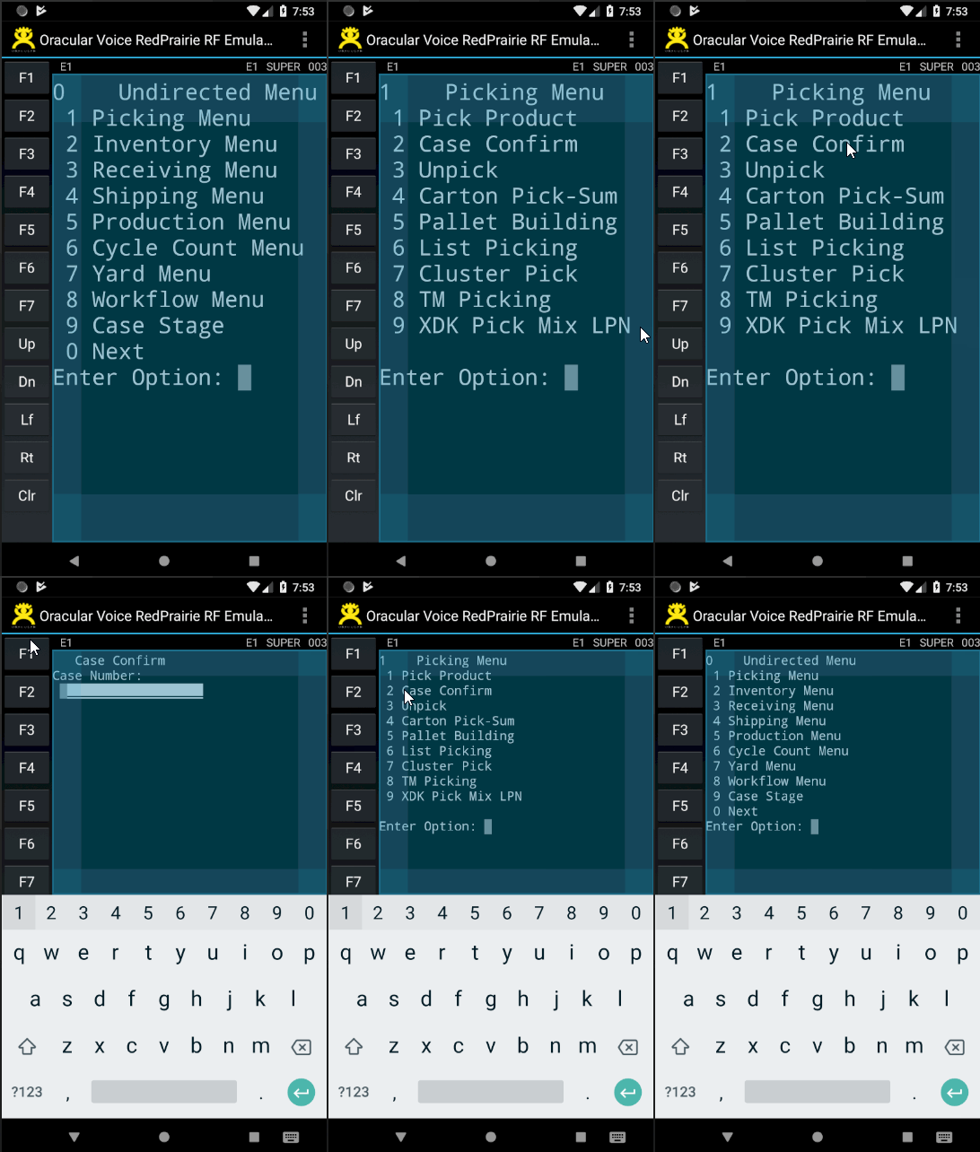
• Function Key pallet is displayed on left side - making it easier to manipulate them.  Refer to the images displayed above to see the function key pallet.
• Soft Keyboard support.  Refer to the image above to see how the soft keyboard appears and disappears
• Automatically Zoom In and Zoom Out to maximize the use of real-estate.  Refer to the image above to see how screen automatically zooms in and out based on the soft keyboard
• Top of the screen provides connection details like environment, user, etc.

• Bottom section of the screen can provide additional contextually sensitive information (described below)

Additional Information

RedPrairie standard RF screens often need to be complimented with additional information.  They do not provide simple ways of providing that so sometimes users would switch to alternate front end with GUI, or have reports.  Our approach in this case is to utilize the full capabilities of the devices and allow users to extend the view with additional information based on the context.  For instance if a pick directs you to a location we could show the inventory in the location along with its attributes like lot, and origin.  We can show multiple pages and the information provided can be different for different users.  The information could be from external sources as well, e.g. ERP or external websites.

This is defined by users themselves and is not a development task.

LES Command Maintenance

We use the les_cmd table to store the commands that are used for this purpose.  This allows us to make changes without needing "mbuild" and thus avoid rollout requirements.  When we execute these commands we always execute the highest level commands - thus providing a mechanism for overriding them as well.

If we want to show a URL then the command returns a special variable called "url":

We have two types of commands - the ones that show data (as shown above) and others that detect the context.  These commands always return one row and one column with a value of 1 or 0:

Additional Information Definition

Additional RF Form Information is defined as a collection.  Several pages may be defined in one collection.  The collection also describes how it fetches the context from the RF form that is running.  The screenshot below indicates that "wrkref" is scrapped from the screen to establish context.  Then three pages will be displayed below the form for additional information.  Each "page" has associated command which would return the data.

Setups

We have defined the various page groupings above.  To use them in a specific context we use the concept of "setups".  Several setups can be defined for an RF form.  Each setup has an associated "condition command" and "Additional Information Id".  The first setup where the conditional command returns true will be used.  This concept can be used to display different types of additional information on same RF form.  For example we could show different data based on type of user or other context information.  A supervisor could, for example, see the inventory levels in the system while doing counting but other users will not.

How it all comes together

When a user goes into an RF form, we check if this form has a setup which is active based on the pre-condition defined.  If there is one we then find the various pages and the associated commands.  We utilize the bottom section of the RF form to show this data where various pages are displayed as tabs and data is displayed in a grid.

Voice Support

If devices support voice, the RF emulator can utilize it as well.  It can speak the form name and the field name.

Conclusion

We have been working with RedPrairie WMS for a long time and understand the intricacies of the architecture.  We also understand the deployment framework and use cases.  This allows us to appreciate the gaps and this solution is based on years of experience in deploying these solutions in various industries and environments.   Once deployed users will appreciate the new capabilities which will result in ease of use and improvement in quality and throughput.  The system support will also become easier.

If you want additional information about this solution or any other Oracular solutions or initiatives contact me at saad.ahmad@oracular.com.  Visit us at http://www.oracular.com

Is Archiving the way to deal with old data in 2018?

Overview

JDA/RedPrairie WMS requires customers to have a data archival strategy. The approach that they push and most customers end up adopting is akin to using a sledge hammer to push a nail.

The JDA approach is quite interesting and probably an appropriate mechanism if the year was 1995. Their approach is to say that the data will be archived to an identical environment from the point of view of software but that other environment will have older data.  This is a very interesting paradigm because all of the reports, queries, use cases, etc. that we may have will work in exactly the same way in the archive environment - all we have to to validate is that the data from the current system is properly moved to the archive instance.

Issues

So what is the issue with above approach?

• We are adding another environment to support.  So lets say we have 5 production environments (for sets of warehouses) - we really need 5 additional environments for archive.  Then to support testing and development we will have 10s of additional environments.  If we have some related environments like EMS, parcel, report writer, etc - those may be needed as well.
• These additional environments need to be part of the software development life cycle.  All rollouts need to go to these environments as well.
• We create "cut off" points, i.e. some queries would need to go to multiple environments.
• Some advanced use cases like "recalling" and "returns" may need overly complex solutions where we may need to query archive and online instances.
• An additional point of failure for daily maintenance.

What are my options?

So do we have any options?  First we really need to check the calendar.  What we considered as "too much data" in 1995 will be considered a "below average database size" today.  Secondly we need to understand that number of rows in a table does not cause an issues - it is the access path.  Thirdly, today's databases have advanced features like partitioning that render such complex strategies obsolete.  In this article, I will focus on solutions available in Oracle - but please note that SQLServer has similar concepts and features.

First let us firmly establish the problem we are trying to solve.  The size of the table is not a measure of performance - it is always the access path - so what we are really trying to address is data management not performance.  Another "problem" that archiving solution supposedly addresses is that queries against the archive instance will not adversely impact the online system's performance.

Data Management - Partitioning

The solution that is most promising for data management problem is to utilize advanced database feature for "partitioning" and let the data stay in the online system.  This implies that your single online instance will have all of the data all the time.  Dispatched shipments will simply be in a different partition.

Ideal partitioning solution will be to create the main partition by range (or in new versions interval partitions).  Then have a sub-partition by warehouse.  That will result in manageable data in each partition.  This partitioning strategy provides good information to the database to parallelize queries.

Data Isolation - Reporting Database

The other problem of providing an isolated environment for queries is easily addressed by utilizing the concept of stand-by database or "data guard" or "reporting databases".  Please refer to the database documentation - but what it provides is a completely isolated database instance that is "almost" up to date and can be used for reporting.  The setup is low level DBA activity and requires little application support.

But this may not be needed for majority of the scenarios.  Such a database should be made available for true research activities where we will not be using the RedPrairie/JDA client to access the tables.  All use cases where we need to access the data through application should be handled by connecting to the online instance and letting database handle the large amounts of data.

How should I partition the data?

To effectively partition we need to have a good date column on the table and for warehouse sub-partition warehouse id should be in the table.  Unfortunately some tables in JDA WMS do not have these columns so small modifications are needed to make it all come together.  

In the following section I have listed the tables and suitable partitioning keys.  Following enhancements should be done to make it all work:

1. When "shipping trailer" dispatches, update following tables with uc_trndte set to dispatch date/time.  And if table does not have a warehouse id, then we set uc_wh_id column.
• trlr
• car_move
• stop
• shipment
• shipment_line
• ord
• ord_note
• ord_line
• ord_line_note
• oub_serv_ord
• oub_serv_ord_line
• pckwrk_hdr
• pckwrk_dtl
• pckmov
• invlod
• invsub
• invdtl
• locmst
• manfst
• shp_dst_loc
• sp_hand_ref
2. When "receiving trailer" dispatches, update following tables with uc_trndte set to dispatch date/time.  And if table does not have a warehouse id, then we set uc_wh_id column.
• trlr
• rcvtrk
• rcvinv
• rcvlin
• locmst
• inb_serv_rcvinv
• inb_serv_rcvlin
3. As a general rule - use base 36 sequences

So the overall partitioning strategy will end up as follows (not including work order tables)

Table	Partition 1	Sub Partition	Online Data	Mod Needed
Transaction History Tables
dlytrn	trndte - month	wh_id - list	No separate concept
trlract	trndte - month	wh_id - list	No separate concept
ordact	trndte - month	wh_id - list	No separate concept
invact	trndte - month	wh_id - list	No separate concept
cnthst	adddte - month	wh_id - list	No separate concept
wrkhst	issdte - month	wh_id - list	No separate concept
canpck	candte - month	wh_id - list	No separate concept
pko_act	ins_dt - month	wh_id - list	No separate concept
pko_act_dtl	ins_dt - month	None	No separate concept
Workflow History Tables
cnfrm_bck_serv	moddte - month	wh_id - list	No separate concept
cnfrm_inv_serv	adddte - month	wh_id - list	No separate concept
cnfrm_noninv_serv	adddte - month	wh_id - list	No separate concept
Order Tables
trlr	uc_trndte-month	stoloc_wh_id	uc_trndte is null	#1
car_move	uc_trndte-month	wh_id	uc_trndte is null	#1
stop	uc_trndte-month	uc_wh_id	uc_trndte is null	#1
shipment	uc_trndte-month	wh_id	uc_trndte is null	#1
shipment_line	uc_trndte-month	wh_id	uc_trndte is null	#1
ord	uc_trndte-month	wh_id	uc_trndte is null	#1
ord_note	uc_trndte-month	wh_id	uc_trndte is null	#1
ord_line	uc_trndte-month	wh_id	uc_trndte is null	#1
ord_line_note	uc_trndte-month	wh_id	uc_trndte is null	#1
oub_serv_ord	uc_trndte-month	wh_id	uc_trndte is null	#1
oub_serv_ord_line	uc_trndte-month	wh_id	uc_trndte is null	#1
pckwrk_hdr	uc_trndte-month	wh_id	uc_trndte is null	#1
pckwrk_dtl	uc_trndte-month	wh_id	uc_trndte is null	#1
pckmov	uc_trndte-month	wh_id	uc_trndte is null	#1
invlod	uc_trndte-month	wh_id	uc_trndte is null	#1
invsub	uc_trndte-month	uc_wh_id	uc_trndte is null	#1
invdtl	uc_trndte-month	uc_wh_id	uc_trndte is null	#1
locmst	uc_trndte-month	uc_wh_id	uc_trndte is null	#1
manfst	uc_trndte-month	uc_wh_id	uc_trndte is null	#1
shp_dst_loc	uc_trndte-month	uc_wh_id	uc_trndte is null	#1
sp_hand_ref	uc_trndte-month	uc_wh_id	uc_trndte is null	#1
Receiving Tables
trlr	uc_trndte-month	stoloc_wh_id	uc_trndte is null	#2
rcvtrk	uc_trndte-month	wh_id	uc_trndte is null	#2
rcvinv	uc_trndte-month	wh_id	uc_trndte is null	#2
rcvlin	uc_trndte-month	stoloc_wh_id	uc_trndte is null	#2
locmst	uc_trndte-month	wh_id	uc_trndte is null	#2
inb_serv_rcvinv	uc_trndte-month	wh_id	uc_trndte is null	#2
inb_serv_rcvlin	uc_trndte-month	wh_id	uc_trndte is null	#2
Job/Task History Tables
job_definition_exec	start_dte-month
task_definition_exec	start_dte-month

Conclusion

If you have been live for some time - chances are you have experienced your share of Archiving Blues. Because of the overly complex archive solution - people often resent even going to archive instance. Volumes of priceless data in dlytrn is completely ignored and rather than valuing it we consider it a burden. Using the simple strategies described here we can enter the 21st century for our JDA WMS systems. We can consider dlytrn as a valuable data source which we choose to not purge and are not worried about it growing to 100s of millions of rows. We can utilize simple techniques like "stand-by databases" and mine through that data to see what gems may be there - or if we do not have time or budget right now at least we can leave data there rather than losing it. Also by keeping it all in one system where historical data is easily accessible we do not have to worry about untimely exceptions. If we have to print a packing slip from 5 years ago - no problem; we simply go to "Report Operations" and print it.

Integrator In-Memory Database - Makes Integration Even Easier

Overview

Recent RedPrairie Integrator versions include an embedded H2 database that opens up new possibilities for efficient and simple integration projects.  The basic components provided are:

• create internal table
• insert into internal table
• select from internal table
• This command asks for a table_name as a parameter - but we can pass a complete join clause as well.
• release internal tables

In some respects the idea is similar to caching discussed in another post - but the added functionality that helps in integration is the ability to apply complete SQL operations.

As of the writing of this blog, this functionality is less known and primarily used internally by RedPrairie integrator itself to abstract the inbound IFD as a table and for "Expression on Child Segment" IFD Field class - but it can come in handy in other cases as well.

Complex Mapping Scenario

If the inbound structure closely matches the RedPrairie concepts - then nothing special is needed - but in some cases the structures can be quite different.  In my experience the various SAP IDOCS present the data in a large number of mutually connected segments, for example:

Here the left side represents an incomplete view of a delivery in SAP.  Right hand side represents an order in WMS.  As you can see the SAP view is a lot more verbose and it needs to transform basically down to a order and order lines.

How to handle this mapping in standard integrator?

This type of mapping is not a problem for Integrator.  It has been able to handle it since the earliest versions.  Some of the tools available are;

• Ability to access any inbound IFD field as an EO Column
• Create EO segments at the same level as inbound IFD
• Using "Expression on Child Segment" concept on the final result IFD.

Some less experienced implementers end up creating intermediate tables to address this type of mapping - that is not needed.  We can map it in one shot, i.e. inbound IFD goes via EO creation to the result IFD which looks like the right hand side.

The result is that the integration works but can be a resource hog.  Basically every time an EO segment instance is created - it has to push a subset of the inbound IFD to the internal database (it used to be actual tables and now it is the embedded H2 database) and then system allows for executing SQL against it.  As described above the traditional solution would have required several EO segments parallel to the various inbound IFD segments, e.g.

Once these additional EO segments have been created - the final result IFD will use "Expression on Child Segment" to create the final fields.  Each of these IFD fields will require integrator to push the EO segment data to the internal database so that SQL can be applied.  Lets say you have 10 order line fields that have to be created in this fashion - it will require the EO data to be pushed to the internal database 10 times for the same order line.  As you can see this can quickly become a performance issue.

Internal Database to the rescue

At a very basic level - the above discussion highlights the key deficiency in integrator - that it does not allow for joining data from multiple inbound segments.  So creating the intermediate EO segments is a way to circumvent that.  Using the internal database we can overcome this and simply load the inbound IFD to internal databases.  Afterwards we can simply join the data so that the EO also matches the result IFD:

The basic difference is that we have introduced a high level segment that would load all of the relevant inbound IFDs to internal database as tables.  And at the end we would release those tables.  The retrieve method implementation of the UC_LOAD_HOST_ORD will utilize the "create internal table" and "insert into internal table" commands.  

First we need to create a component that would return a resultset for each inbound IFD segment that we are interested in. For example lets call that component "get usr sap order segments as rs". It could be implemented as:

/*
 * During integrator execution - ifd_data_ptr is on stack
 * so it does not need to parse the inbound again.  But
 * in case it is not on stack, e.g.
 * for testing then we get it via standard
 * integrator command.
 */
if ( @ifd_data_ptr#onstack )
   hide stack variable where name = 'ifd_data_seq'
else
   sl_get ifd_data_ptr 
|
{
   /*
    * If an inbound IFD is optional - we need to still
    * create an empty recordset for it
    */
    ... create empty recordsets
    |
    /*
     * Now fetch the inbound IFD Data into a
     * recorset, e.g. lets say inbound IFD
     * segment is called MYSAPHDR - we will say
     */
   {
      {
         sl_list ifd_data_fld <
         where ifd_seg_id = 'MYSAPHDR'
         >> uc_sap_mysaphdr
      }
   }
   |
   ... so on.  Get every relevant inbound IFD
   ... segment to a recordset.
   ... This step is extremely efficient as it
   ... is simply looking at parsed 
   ... view of inbound IFD from memory.  
   ... If an inbound IFD was optional, e.g.
   ... order notes - then you still need
   ... to create a valid recordset with 1 row.
}

Now we can create another command say "create usr sap order tables" as follows:

get usr sap order segments as rs
|
{
   release internal tables
   ;
   create internal table
   where table_name = 'uc_sap_mysaphdr'
   and res = @uc_sap_mysaphdr
   ;
   ... so on for all tables
}

The UC_RELEASE_HOST_ORD will simply call "release internal tables" command.

With that in place the ORDER_HDR, ORDER_DETAIL etc. will no longer utilize the generated retrieve method implementation that says "where sl_data_fk = :sl_data_pk" instead it will call a MOCA Command  that will utilize "select from internal table" to get data from multiple inbound IFD segments utilizing joins - which is extremely efficient.

This will utilize the several tables created earlier and access the data from there. It can utilize complete SQL language including group and join clauses:

{
   select from internal table
   where select_stmt =
     "select ... any columns from any table ...."
   and table_name = 
     " uc_sap_mysaphdr join .. left outer join .." 
}

Some Gatchas

• Note that the internal tables are created directly from the recordset.  If the recordset is empty, the table cannot be created as it does not have the column information.  That is why we need to have an empty table in that case.  The "sl_list ifd_data_fld" command returns ifd_data_seq and ifd_data_dtl_seq in the recordset.  So you can create the empty recordset with these values set as 0.  That way the recordset will not be empty but when you access it for the particular ifd_data_seq you will not get a row - which is what we wanted.
• If this functionality is used, then all segments below UC_LOAD_HOST_ORD must use this and not the traditional "sl_data_fk = :sl_data_pk" retrieve methods.  This is because when creating the tables we called "release internal tables" and that also killed the table that integrator had created for this SQL to work.
• Referring to first gotcha - note that in MOCA if you assign one recordset to another, it just sets the pointer and does not clone the data.  This implies that if you set multiple recordsets to the same "empty" recordset then even though you are thinking they are two different recordsets - they are really the same.  So if you move to the last row in one - you will also move to the last row in the other.  Where it would cause an issue is that when you will create the internal table from one - the next one will not work.  You will need to call ".reset" on the recordset again before using it.

Summary

The basic idea is that we should try to match event output to the RedPrairie order model via this capability.  That implies that we push the inbound data to in-memory tables once and then join them as needed to create the final set.  At a very high level the approach is similar to a two-step approach of first loading the data to temporary staging area and then logging another event from that - but this achieves that in a single step and will be more optimal - both in performance and also in management.

Right way to tackle RedPrairie/JDA Interfaces

Every WMS implementation needs to deal with interfaces.  This includes host interfaces, e.g. interfacing with SAP, Oracle, JDE, etc. and also to the automation equipment.  Many times the project plan calls for these tasks at the wrong time and that can lead to overall delays and rework.  Timing this activity correctly is critical to the overall success of the project.

Many times the customer's past experience with interfacing influences their decision to start interface discussion prematurely - but such proactive approach is not helpful.  So one thing we need to establish upfront is that RedPrairie/JDA will be able to handle any type of interface requirement.  If you can send it RP can process it! So do not lose your sleep over it.

Abstraction is the key

We need to understand that the actual project is WMS implementation and not the interfaces.  Interfaces need to be understood abstractly as just another mechanism to provide data.  Nothing more and nothing less.  So once it is established that RP can do any type of interface work then we need to focus on WMS solution summary and not interfaces.  

Proper place for Interfaces in the Project Plan

At a very high level, the project plan should be as follows:

1. Key customer resources get trained on the solution set.
2. Software is installed in development environment
3. A Proof of Concept exercise is done with standard solution
1. This highlights the interfaces
4. A solution summary is developed
1. Interfaces are called out here
5. Interface Discussion

A completely wrong approach will put the interface discussion ahead in the plan.  I have seen instances where the interface discussion is done even before the software is installed.  Such meetings are not very productive because the customer's resources do not understand RP and the implementer does not understand customer requirements - so as a result a sub-par interface diagram is created.

Host Interface Matrix

Host interfaces are simply a mechanism to provide data to RedPrairie.  It is not different from manual data entry from that aspect.  Solution summary should be firmly established before this discussion starts.  One way to approach this is that the customer could simply take screenshots from RedPrairie client and highlight the data that they expect to come from a host system - that will be easier than going through spreadsheets with cryptic column names.  Any RP implementer should be able to take such a document and convert that to an actual interface.

Similarly for data going to host, the customer SME (Subject Matter Expert) can highlight the data that they would expect to populate the host system.

MHE Interfaces

MHE (Material Handling Equipment) interfaces are no exception.  The full solution summary should first describe the use cases in terms of RF flows.  This should be done even if majority of the picking is done by MHE.  This provides a baseline for testing.  Once this is done, MHE use cases should be defined and an equivalence diagram should be created.   This diagram will describe how MHE picking, for example, is equivalent to RF picking.  A diagram like this will form the basis for MHE interface discussions.  This will also help during development and unit testing phases.

MHE Emulator

Ability to emulate MHE messages is key to a successful implementation.  Unfortunately many MHE systems do not provide such capability.  This becomes a challenge if MHE system communicates over sockets.  A simple emulator can be created by RedPrairie integrator where you can create a system that represents the host system and listens for messages.  You can verify MHE protocol in this way.  You can use similar techniques to send completion messages back to WMS. 

When sending data to MHE, typical triggering point is the pick release process.  pckwrk table(s) should form the basis for data that is sent to MHE for picking.  Custom columns can be added here to incorporate any unique concepts but this should generally be the starting point.

The transactions back from MHE will typically call a flavor of "move inventory".  If we have an equivalence of these use cases to RF screens then this can be a relatively simple exercise.

Another approach may be to have a folder with raw messages and create a simple groovy command that sends data from this folder to the WMS.  You can also use "telnet" to send data.

Interesting WMS Concepts for MHE

RedPrairie WMS provides several concepts that can form the basis for providing data to MHE at proper level.  Often I have seen that new concepts are introduced in this regard which adds needless complexity and testing headaches:

• Idea of picking cartonization
• Idea of lists that can group cartonized cartons
• Non cartonized picking directly to a tote
• Pick Release process and associated standard triggering points like "register picks released"
• Replenishment Configuration concepts

For most picking systems, e.g. Pick To Light, the MHE system will have a location table with similar locations as RedPrairie.  Inventory levels in RedPrairie will be assumed to be accurate as well.  In such systems orders are allocated within RedPrairie and at pick release time we send data to the MHE system.  RedPrairie concepts are a "shoe in".  By the time pick release is done - we know exactly which carton needs inventory from which MHE locations so appropriate messages can be constructed.

When MHE system completes a pick - some systems will tell exactly what was picked while some will simply say "this tote is picked".  In either case - processing of such a message should simply call "move inventory".  Sometimes implementer would make this interface needlessly complicated by a false assumption that "move inventory will be too expensive".  This unproven and untested notion will then translate to new concepts and make the whole implementation overly complicated.  It is always best to not over-engineer this step and simply pick the inventory in RedPrairie when it is picked in MHE.

MHE system from this point on may have multiple stops, e.g. audit station, weight station, etc.  Such locations may be handled as simple P&D locations or hops.  In either case - if MHE system can send a message in these cases - that message should translate into a "move inventory" call.  Refer to this article if you have a use case where certain percentage of totes need to be audited.

Every implementation may be slightly different but always have following goals:

• Do not invent new concepts
• Always equate to corresponding RF use cases

Summary

Interfacing capabilities are a strong suit for RedPrairie/JDA WMS systems.  Do not let some bad past experiences influence the project plan too much.  Considering interfaces as just another type of data entry method simplifies the project a great deal.  Based on the type of implementation - you may need significant hours, but those should not translate to significant complexity.  Proper abstraction that preserves the core RedPrairie concepts will go a long way.